Ray Intersection Points

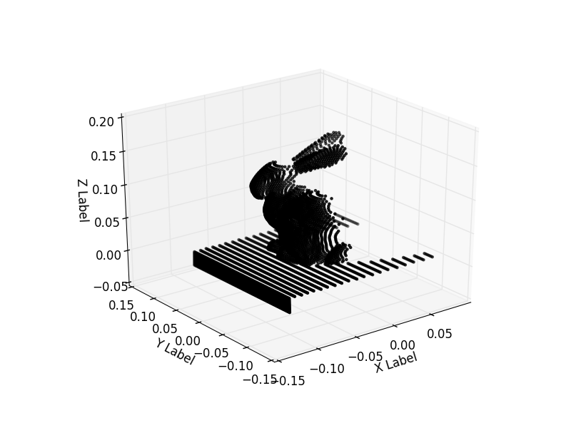
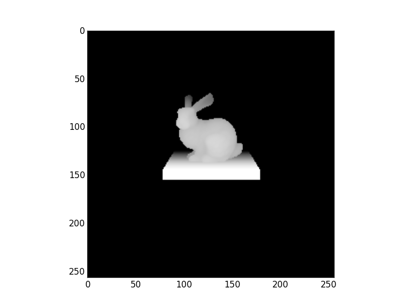
Rays are launched in the same way as the pinhole camera. The simple scene consists of the Stanford bunny model sitting on a platform. For every ray that is launched, the cartesian hit point of the ray with the materials in the scene (rabit and floor) is recorded. In Figure 1 the 3D hit point for each ray in the camera is plotted in 3D space. In Figure 2 the z coordinate of each hit point is scaled and plotted to indicate distance from the camera. Both methods allow simple visualisation of a scene and extraction of intersection geometry data.

Bunny model source:

Stanford University Computer Graphics Laboratory http://graphics.stanford.edu/data/3Dscanrep/ Converted to obj format using MeshLab

# External imports
from os import path
from numpy import tan, pi as PI
import numpy as np
import matplotlib.pyplot as plt

# do not remove the following import or the 3D plotting will break
from mpl_toolkits.mplot3d import Axes3D

# Internal imports
from raysect.core.ray import Ray as CoreRay
from raysect.optical import World, translate, rotate, Point3D, d65_white, ConstantSF, Node, Vector3D
from raysect.optical.material.emitter import UniformVolumeEmitter
from raysect.optical.material import Lambert
from raysect.primitive import Box, Subtract
from raysect.primitive.mesh import Mesh
from raysect.optical.library import schott


"""
A demo of Ray intersection hit points
----------------------------------

Rays are launched in the same way as the pinhole camera. The simple scene consists
of the Stanford bunny model sitting on a platform. For every ray that is launched,
the cartesian hit point of the ray with the materials in the scene (rabit and floor)
is recorded. In Figure 1 the 3D hit point for each ray in the camera is plotted in
3D space. In Figure 2 the z coordinate of each hit point is scaled and plotted to
indicate distance from the camera. Both methods allow simple visualisation of a
scene and extraction of intersection geometry data.

Bunny model source:
  Stanford University Computer Graphics Laboratory
  http://graphics.stanford.edu/data/3Dscanrep/
  Converted to obj format using MeshLab
"""

world = World()

mesh_path = path.join(path.dirname(__file__), "../resources/stanford_bunny.rsm")
mesh = Mesh.from_file(mesh_path, parent=world, transform=rotate(180, 0, 0))

# LIGHT BOX
padding = 1e-5
enclosure_thickness = 0.001 + padding
glass_thickness = 0.003

light_box = Node(parent=world)

enclosure_outer = Box(Point3D(-0.10 - enclosure_thickness, -0.02 - enclosure_thickness, -0.10 - enclosure_thickness),
                      Point3D(0.10 + enclosure_thickness, 0.0, 0.10 + enclosure_thickness))
enclosure_inner = Box(Point3D(-0.10 - padding, -0.02 - padding, -0.10 - padding),
                      Point3D(0.10 + padding, 0.001, 0.10 + padding))
enclosure = Subtract(enclosure_outer, enclosure_inner, material=Lambert(ConstantSF(0.2)), parent=light_box)

glass_outer = Box(Point3D(-0.10, -0.02, -0.10),
                  Point3D(0.10, 0.0, 0.10))
glass_inner = Box(Point3D(-0.10 + glass_thickness, -0.02 + glass_thickness, -0.10 + glass_thickness),
                  Point3D(0.10 - glass_thickness, 0.0 - glass_thickness, 0.10 - glass_thickness))
glass = Subtract(glass_outer, glass_inner, material=schott("N-BK7"), parent=light_box)

emitter = Box(Point3D(-0.10 + glass_thickness + padding, -0.02 + glass_thickness + padding, -0.10 + glass_thickness + padding),
              Point3D(0.10 - glass_thickness - padding, 0.0 - glass_thickness - padding, 0.10 - glass_thickness - padding),
              material=UniformVolumeEmitter(d65_white, 50), parent=light_box)


fov = 45
num_pixels = 256


# Launch rays using the same geometry calculations as a pinhole camera
image_width = 2 * tan(PI / 180 * 0.5 * fov)
image_delta = image_width / num_pixels

image_start_x = 0.5 * num_pixels * image_delta
image_start_y = 0.5 * num_pixels * image_delta

x_points = []
y_points = []
z_points = []
z_show = np.zeros((num_pixels, num_pixels))
for ix in range(num_pixels):
    for iy in range(num_pixels):

        # generate pixel transform
        pixel_x = image_start_x - image_delta * ix
        pixel_y = image_start_y - image_delta * iy

        # calculate point in virtual image plane to be used for ray direction
        origin = Point3D().transform(translate(0, 0.16, -0.7) * rotate(0, -12, 0))
        direction = Vector3D(pixel_x, pixel_y, 1).normalise().transform(translate(0, 0.16, -0.7) * rotate(0, -12, 0))

        intersection = world.hit(CoreRay(origin, direction))

        if intersection is not None:
            hit_point = intersection.hit_point.transform(intersection.primitive_to_world)
            x_points.append(hit_point.z)
            y_points.append(hit_point.x)
            z_points.append(hit_point.y)
            z_show[iy, ix] = hit_point.z
        else:
            # add small offset so background is black
            z_show[iy, ix] = 0.1

fig = plt.figure()
ax = fig.add_subplot(111, projection='3d')
ax.scatter(x_points, y_points, z_points, c='k', marker='.')
ax.set_xlabel('X Label')
ax.set_ylabel('Y Label')
ax.set_zlabel('Z Label')

plt.figure()
plt.imshow(z_show, cmap=plt.cm.Greys)

plt.show()

The 3D intersection point of each camera ray with the materials in the scene is recorded and plotted as 3D points.

The Z coordinate of each intersection point is scaled and plotted to indicate distance from the camera. This allows a crude form of scene visualisation.